Developers Dairy: creating a multi-level Dependent Drop-down lists in Excel

The sheet below allows users to select a country, a corresponding state and city.

Once a country is selected, the “State\Region\Province” Column is filtered to return only the states of the country selected as shown below:

Similarly, once a state is selected, the “City\County\District” column is filtered to return only the cities of the state selected as shown below:

Column B and C uses the dependent drop-down functionality. See below how to implement this functionality in your related lists.

Steps to create a multi-level dependent drop-down list

1.Prepare the dataset
In this example, we are using a geographical dataset having a list of countries, states and cities. We have pulled in this data from Azure SQL Database. You can use any other related lists.

Below is the sample dataset:

Full data table showing geographical data across the globe

2. Prepare a unique list for level 1

You will need to have a unique list for the first level. This is the column that other columns will depend on. In this example, the first level is column A (the Country column).

Image showing the 3 levels (columns A, B and C)

To create the unique list, we added a new sheet and named it “State lookup”. In this sheet we use the unique function to return a unique list form the Full data table shown in step 1

Below is the list of unique countries.

3. Set up the data validation for level 1

After you have made a unique list of level 1, the next step is to set up the data validation for that level.

Here we will rebuild the sample solution from scratch. Have created a new sheet and have named the columns appropriately with some colours as well.

We will now proceed to add a data validation on column A (level 1to aid user entries. To add a data validation,

· select as many cells as you want to add the data validation to. We have selected cells A2 to A10

· Next, on the Excel ribbon click on data validation.

This will open the data validation box:

· On the settings tab click on the selection box and select “List”

· Next on the source box, click on the arrow to select where the list should get its data from.

Click enter once you have selected the entire range of your data

· Click on Ok. Level 1 now has a drop-down list.

Setting up data validation list for level 1

4. Set up the first dependent drop-down list

With level 1 completed, we will then proceed to create our first dependent drop-down list. In this example that will be on the column B (the State column). We want to create a list of states that will be dependent on the country selected in level 1.

To do this, on the sheet having your 3 levels, select column D2 and put this formula:
= FILTER (State,Country = Dashboard!A2, "")

The FILTER function in Excel filters a range of data based on specified criteria. The result is an array of values that automatically spills into a range of cells.

In this example, FILTER (State,Country = Dashboard! A2, ""))

State – This is the range being filtered. In this example it is the state column in the full data table.

Country = Dashboard! A2 – This is the criteria for the filtering.

“” – this makes the filter function return an empty string when there is no result.

In this example we are saying filter the state column in the full data table and return a list of only where the country column in the raw data is equal to the country selected in your sheet. And if no country is selected, let it return an empty string.

We have put the formular in cell D2 and just as the formula says, it returns nothing when no country is selected. Now we will select a country and see the output of the formula

Selecting a country for row 2 to see output of the filter function

As shown from the above, when a country is selected, the filter function returns a vertical list of only the state belonging to the country selected. But we noticed the result comes with repetitions just as it is in the full data table. That’s where the unique function comes in.

The Excel UNIQUE function returns a list of unique values from a range or array of data.

So, we put the filter function inside the unique function to return the distinct states. =UNIQUE (FILTER (State, Country = Dashboard! A2, "")).

Distinct list of states in United States

The last function is the TRANSPOSE function. As seen above, the filter function returns a “Vertical” list. This is a bit problematic when you want to work with more than one row. To illustrate this, let’s use this vertical array to create a dependent drop-down list on the state column for cells B2 to B10.

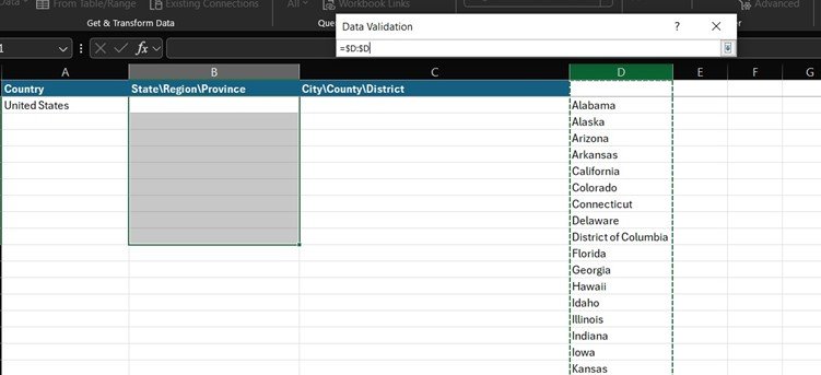
To do this, we select cells B10 then click on data validation and select column D as the source for the drop-down list.

As we can see, when the country is United states, we see only states belonging to the United States. Next, we change the country and see that the state loop up list changes as well. Notice, column D is changing as well. So, column B is dependent on level 1.

Next, let’s select Canada in row A2 and a state say Ontario in row B2.

Then, let’s select another country in column A3 say United States and then let’s select a state in the US say Alabama

Oops, you notice that although we have another country in row 3 (United States), the drop-down for the state is still showing states for Canada and same for the source in column D. So, although it works well for row 2 it is not working for row 3. This is the issue with the vertical array returned by the filter function. It becomes problematic when you want to implement the dependent-drop down functionality in multiple rows. Hence, we want the array returned by the FILTER function to be a horizontal list instead so that each row will have its own array and as such we will be able to tie each row to its own list. This is where the TRANSPOSE function comes in.

The TRANSPOSE function in Excel changes the direction of a range or array of data, converting horizontal data to vertical and vice versa.

So, we will put in the unique and filter function inside of a transpose so the array returned will be horizontal.

=TRANSPOSE(UNIQUE(FILTER(State,Country = Dashboard!A2, "")))

TRANSPOSE function added to the formula in column D to return horizontal list

We will now drag the formula in the source column D to as many rows as we want in this case to D10

As we see, in row 3, the array returned is states in United states. For rows where there is no country selected, it returns empty as specified in the filter function.

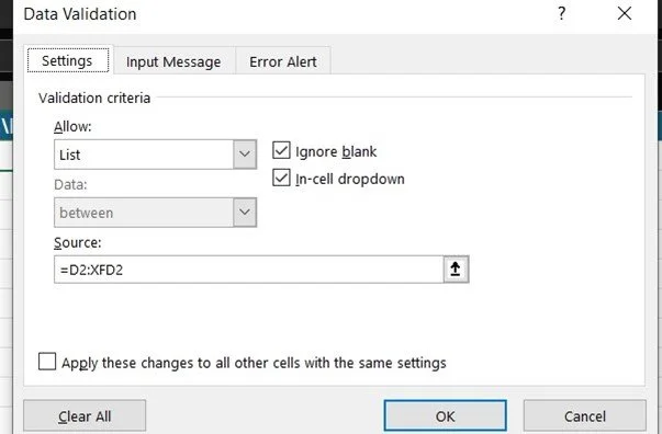
Next, we will then edit the data validation for the state to now pick its source from the horizontal list instead of the vertical list. To do this we select cell B2 then click on data validation and then change the source.

Since the length of data for each row will vary, we will select as much columns possible, in our example: $D$2:$XFD$2

Next, we will edit the source and remove the $ signs. This way we will be able to drag it and apply the formula to other rows.

Click Ok.

Next, drag the drop-down to as many rows in this case we will drag to cells B10.

We will now select states for each and see the result.

In row 2 we have selected Canada in A2; we see the state, B2 is filtered for states in Canada alone

In row 3 we have selected United States in A3; we see the see the state in B3 is filtered for states in United States alone and same goes for row 4 where we have selected China in A4. We can see the dynamic list for each row at the left as well.

Dependent drop-down across multiple rows

So, using the TRANSPOSE function, we have resolved the issue we had using the vertical array returned by the FILTER function. We now have a dynamic dependent drop-down list for column B that works across multiple rows.

5. Set up the next dependent drop-down list

We will now do same for column C (level 3, the city column). We will create a list that depends on column B. That is, column C will only contain cities for the country selected in column B. In this sample solution, to keep the front user sheet tidy, we have done the cities lookup list in a different sheet.

After setting up the cities look up source sheet. We will now go to the main sheet.

On the main sheet select cell C2 then click on data validation and specify the source to be the cities look up sheet.

We will remove the $ signs so that we can copy the drop down to other rows.

We will now select cities for the states above.

Selecting a city in California, United States

Selecting a District\Province in Shanghai, China.

Column C is a multi-level dependent drop-down list since it depends on the state list which in turn depends on the country list.

We will now tidy up the main sheet by moving the state look up list in column D to another sheet as we did with the cities look up list.

The final solution looks like this:

State drop-down list that is dependent on country selected on each row

Cities drop-down list that is dependent on state selected on each row